Serial Correlation Removal

In this section, you will learn to remove Serial Correlation from dataset in STATA. We will explain in detail about them in the following steps:

Let us assume, the name of the MS-Excel datasheet is "Time-Series-Data-Representation.xlsx" and it is located in the path "D:\data\". Then the data upload command in STATA is given by:

import excel "D:\data\Time-Series-Data-Representation.xlsx", sheet("DATA") firstrow

Now click ENTER. Your data is uploaded in STATA.

Once the data is uploaded in STATA, we need to define the data to be time series data. For that purpose, we need to declare the time-series id in the data. Then the data declaration command in STATA is given by:

tsset YEAR

Once you click ENTER, you will get the following:

time variable: YEAR, 1971 to 2010
delta: 1 unit

Now your data is declared in STATA.

Once the data is declared in STATA, you can check for serial correlation. In order to check serial correlation, first you will have to run a regression on the variables, so that residuals of the regression can be generated. In the dataset, there are three variables (EC, CE, and GDP).

Let us assume that CE is the dependent variable, EC and GDP are independent variables. Now, first we will run the OLS regression. Then the command in STATA is given by:

regress CE EC GDP

Once you click ENTER, you will get the following:



So, we have the results for the OLS regression. Now, we need to check for the serial correlation in the residuals. For this purpose, we will run the Breusch and Godfrey LM test on the residuals. The basic command for performing orthogonal transformation in STATA is estat bgodfrey. The command in STATA is given by:

estat bgodfrey, lags(1)

Once you click ENTER, you will get the following:



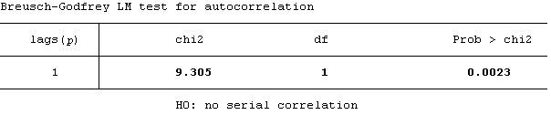
So, we have the results for the Breusch-Godfrey LM test. Here we can see that the Prob > chi2 value of chi2 statistic is significant at 1% level. It indicates that the residuals are not free from serial correlation, after 1 lag. This can be tested for any number of lags. For instance, we will check for serial correlation after 9 lags. The command in STATA is given by:

estat bgodfrey, lags(9)

Once you click ENTER, you will get the following:



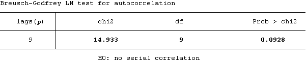
Here we can see that the Prob > chi2 value of chi2 statistic is significant at 10% level. It indicates that the residuals are not free from serial correlation, even after 9 lags.

By far, we have tested that there is problem of serial correlation in the data. In order to remove that, we take several ways. Here, we will show you two ways of removing it.

In the first method, we will use the lagged value of dependent variable as an independent variable in the OLS regression model. So, let us assume that the lagged value of CE is LCE. We need to create this variable. The command in STATA is given by:

generate LCE = CE[_n-1]

Once you click ENTER, you will get the following:

(1 missing value generated)

Now, you will have to run the OLS regression model using CE as the dependent variable, and EC, GDP, LCE as independent variables. The command in STATA is given by:

regress CE EC GDP LCE

Once you click ENTER, you will get the following:



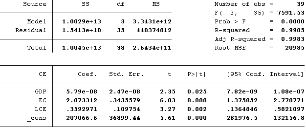
So, we have the results for the OLS regression. Now, we need to check for the serial correlation in the residuals. For this purpose, we will run the Breusch-Godfrey LM test. The command in STATA is given by:

estat bgodfrey, lags(3)

Once you click ENTER, you will get the following:



Here we can see that the Prob > chi2 value of chi2 statistic is statistically insignificant. It indicates that the residuals are free from serial correlation, after 3 lags. Let us check it again with 1 lag. The command in STATA is given by:

estat bgodfrey, lags(1)

Once you click ENTER, you will get the following:



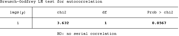
Here we can see that the Prob > chi2 value of chi2 statistic is significant at 10% level. It indicates that the residuals are not free from serial correlation, after 1 lag.

We can see that this method is not always effective for removing serial correlation. Therefore,we will now move towards the second method.

In the second method, we will use the first differentiated values of all the variable in the OLS regression model. So, let us assume that the differentiated value of CE is DCE, EC is DEC, and GDP is DGDP. We need to create these variables. The command in STATA is given by:

generate DCE = CE-CE[_n-1]
generate DEC = EC-EC[_n-1]
generate DGDP = GDP-GDP[_n-1]

Once you click ENTER, you will get the following:

(1 missing value generated)
(1 missing value generated)
(1 missing value generated)

Now, you will have to run the OLS regression model using DCE as the dependent variable, and DEC and DGDP as independent variables. The command in STATA is given by:

regress DCE DEC DGDP

Once you click ENTER, you will get the following:



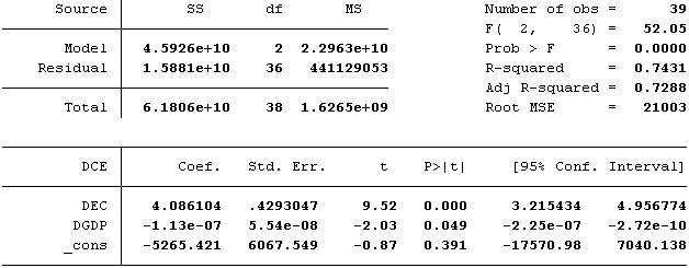
So, we have the results for the OLS regression. Now, we need to check for the serial correlation in the residuals. For this purpose, we will run the Breusch-Godfrey LM test. The command in STATA is given by:

estat bgodfrey, lags(1)

Once you click ENTER, you will get the following:



Here we can see that the Prob > chi2 value of chi2 statistic is statistically insignificant. It indicates that the residuals are free from serial correlation, after 1 lag. Just to make sure, we will run this test for 3 lags. The command in STATA is given by:

estat bgodfrey, lags(3)

Once you click ENTER, you will get the following:



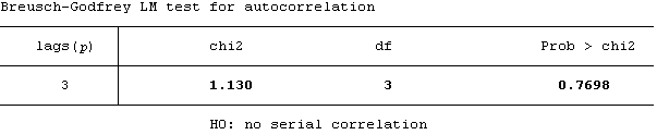
Here we can see that the Prob > chi2 value of chi2 statistic is statistically insignificant. It indicates that the residuals are free from serial correlation, even after 3 lags. So, we can say that the test results are free from serial correlation.

Following these steps, you can easily check and rectify the problem of serial correlation in STATA. For more information on these tests and carrying out other tests for checking serial correlation, please give the following command in STATA:

help estat bgodfrey

If the bgodfrey command is not installed in STATA, then you will have to use the following command in STATA to find and install the code:

findit estat bgodfrey