Panel Unit Root Test

In this section, you will learn to carry out the panel unit root tests (IPS, LLC, ADF, Breitung, and others) in STATA. We will explain in detail about them in the following steps:

Let us assume, the name of the MS-Excel datasheet is "Panel-Data-Representation.xlsx" and it is located in the path "D:\data\". Then the data upload command in STATA is given by:

import excel "D:\data\Panel-Data-Representation.xlsx", sheet("DATA") firstrow

Now click ENTER. Your data is uploaded in STATA.

Once the data is uploaded in STATA, we need to define the data to be panel data. For that purpose, we need to declare the cross-section and time-series ids in the data. Then the data declaration command in STATA is given by:

xtset CODE YEAR

Once you click ENTER, you will get the following:

panel variable: CODE (strongly balanced)
time variable: YEAR, 2001 to 2013
delta: 1 unit

Now your data is declared in STATA.

Once the data is declared in STATA, you can run the unit root tests. The basic command for running a unit root test in STATA is xtunitroot. It has different options of running ADF, LLC, IPS, Breitung, and other tests individually. In the dataset, there are five variables (POP, EC, PT, Y, and N). Now, let us assume, you want to test the ADF unit root for the variable Y at the level. Then the command in STATA is given by:

xtunitroot fisher Y, dfuller lags(1)

Once you click ENTER, you will get the following:



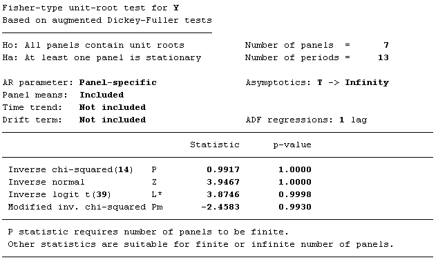
Now, please note that we have included lags(1) in the command. You can also adjust the lag length according to your convenience and requirement of the study. One thing you need to notice here, that the results are indicating the presence of unit root in Y (look at the p-value of Modified inv. chi-squared).

Now, let us assume, you want to test the LLC unit root for the variable Y at the level. Then the command in STATA is given by:

xtunitroot llc Y

Once you click ENTER, you will get the following:



Now, this command is comparatively straightforward compared to the previous one. In this case also, you can adjust the lag length like the previous one. In this case also, the results are indicating the presence of unit root in Y (look at the p-value of Adjusted t*).

Now, let us assume, you want to test the IPS unit root for the variable Y at the level. Then the command in STATA is given by:

xtunitroot ips Y

Once you click ENTER, you will get the following:



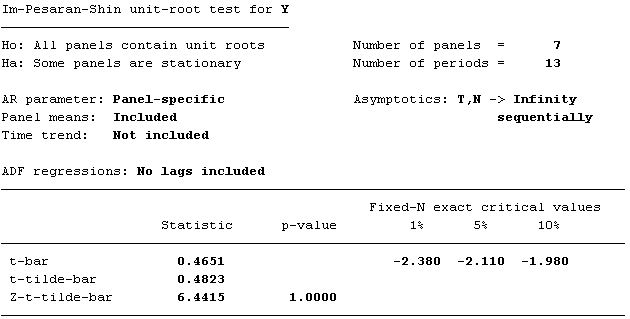
In this case also, you can adjust the lag length. Like the previous two cases, the results are indicating the presence of unit root in Y (look at the p-value of Z-t-tilde-bar).

Now, let us assume, you want to test the Breitung unit root for the variable Y at the level. Then the command in STATA is given by:

xtunitroot breitung Y

Once you click ENTER, you will get the following:



In this case also, you can adjust the lag length. Like the previous three cases, the results are indicating the presence of unit root in Y (look at the p-value of lambda).

By far, we have tested that the variable Y has unit root at the level. Now, we need to check, whether this variable contains unit root after first difference, or not. For most of the statistical analysis techniques involving unit root tests, it is required that the variables should be stationary at least after first difference. For that purpose, first we need to differentiate the variable, and we will store the differentiated values in a new variable, named DY. Then the command in STATA is given by:

by CODE: generate DY=Y-Y[_n-1]

Once you click ENTER, you will get the following:

(7 missing values generated)

Now that we have generated the differentiated variable, we can now proceed with the unit root tests, just like we have just mentioned. So, let us start with the ADF test. The command in STATA is given by:

xtunitroot fisher DY, dfuller lags(1)

Once you click ENTER, you will get the following:



Now, please notice here, that the results are indicating that the unit roots in Y are removed (look at the p-value of Modified inv. chi-squared).

Now, we will apply the LLC unit root for the variable DY. The command in STATA is given by:

xtunitroot llc DY

Once you click ENTER, you will get the following:



Now, please notice here, that the results are indicating that the unit roots in Y are removed (look at the p-value of Adjusted t*).

Now, we will apply the IPS unit root for the variable DY. The command in STATA is given by:

xtunitroot ips DY

Once you click ENTER, you will get the following:



Now, please notice here, that the results are indicating that the unit roots in Y are removed (look at the p-value of Z-t-tilde-bar).

Now, we will apply the Breitung unit root for the variable DY. The command in STATA is given by:

xtunitroot breitung DY

Once you click ENTER, you will get the following:



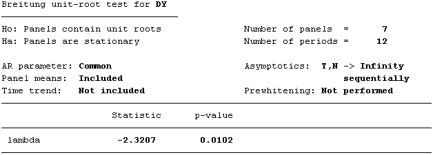
Now, please notice here, that the results are indicating that the unit roots in Y are removed (look at the p-value of lambda).

Following these steps, you can easily carry out the panel unit root tests in STATA. For more information on these tests and carrying out other panel unit root tests, please give the following command in STATA:

help xtunitroot

If the xtunitroot command is not installed in STATA, then you will have to use the following command in STATA to find and install the code:

findit xtunitroot