GMM Analysis


In this section, you will learn to carry out the GMM (Generalized Method of Moments) analysis in STATA. We will explain in detail about this in the following steps:


Step 1: Upload the MS-Excel datasheet in STATA


Let us assume, the name of the MS-Excel datasheet is "Panel-Data-Representation.xlsx" and it is located in the path "D:\data\". Then the data upload command in STATA is given by:

import excel "D:\data\Panel-Data-Representation.xlsx", sheet("DATA") firstrow

Now click ENTER. Your data is uploaded in STATA.


Step 2: Define the data as panel data in STATA

Once the data is uploaded in STATA, we need to define the data to be panel data. For that purpose, we need to declare the cross-section and time-series ids in the data. Then the data declaration command in STATA is given by:

xtset CODE YEAR

Once you click ENTER, you will get the following:

panel variable: CODE (strongly balanced)
time variable: YEAR, 2001 to 2013
delta: 1 unit


Now your data is declared in STATA.


Step 3: Run the GMM estimation in STATA


Once the data is declared in STATA, you can run the GMM estimation. The basic command for running a GMM estimation in STATA is gmm. It has different options of running step-wise and iterative estimations individually. In the dataset, there are five variables (POP, EC, PT, Y, and N), and for the purpose of analysis, we can assume Y as dependent variable, POP and EC as independent variables, and PT and N as the instrumental variables. Here, we are considering POP as the exogenous variable. While choosing instruments, you should always remember this: No. of instruments >= No. of exogenous variables. So, the command in STATA is given by:

gmm (Y-{b1}*POP-{b2}*EC-{b0}), instruments(PT N)

Once you click ENTER, you will get the following:


Now, look at the individual coefficients. The coefficient of POP is statistically insignificant, the coefficient of EC is significant at 1% level (look at the
p-values of the coefficients). The instrumental variables are shown below the estimation results.


Step 4: Run the diagnostic tests for GMM in STATA


Once we have estimated the GMM, we need to check two things:

  • whether the chosen instruments are proper, or not, and
  • whether there is any problem of overidentification, or not.

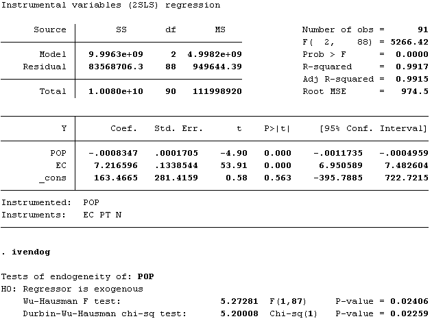
    First, we will check the DWH test for checking the suitability of instruments. This test requires an instrumental variable regression on the same parameters. So, the command in STATA is given by:

    ivreg Y EC (POP = PT N)
    ivendog


    Once you click ENTER, you will get the following:


    Now, notice the
    p-value of Durbin-Wu-Hausman chi-sq test. It is significant at 5% level. It indicates that the choice of instrumental variables has been perfect. This statistic should always be statistically significant.

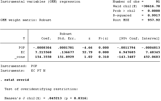
    Next, we will check the Hansen's J test for checking the overidentification problem of the model. This test requires an instrumental variable regression on the same parameters using GMM estimators. So, the command in STATA is given by:

    ivregress gmm Y EC (POP = EC PT N)
    estat overid


    Once you click ENTER, you will get the following:


    Now, notice the
    p-value of Hansen's J chi2(1). It is highly insignificant. It indicates that the model does not suffer from overidentification problem. This statistic should always be statistically insignificant.

    Following these steps, you can easily carry out the GMM analysis in STATA. For more information on these tests and exploring other options of GMM estimation and the diagnostic tests, please give the following commands respectively in STATA:

    help gmm

    help ivreg

    help ivregress

    help ivendog

    help estat overid


    If the commands are not installed in STATA, then you will have to use the following commands respectively in STATA to find and install the codes:

    findit gmm

    findit ivreg

    findit ivregress

    findit ivendog

    findit estat overid


    Go Backfast_rewind
  • add